
Agents are not thinking: Science of agent behavior
Prologue
This is Part 2 of Agents are not thinking, they are searching. Part 1 reframed what agents are (their nature). This part builds the instruments for studying them. This essay is less theory and more code (even math for anyone liking formalism enough). This essay will have follow ups given how much fun I have had making it ; but they will come after i let myself soak more with the idea.
The limits of my language mean the limits of my world — Ludwig Wittgenstein
The nature of a thing is more important than its form. — Brok
technoyoda/aft a toolkit for studying agent behavior →
My previous essay was a spinal response, an attempt to jot down the intuition behind how agents actually behave. But once the intuition was expressed, it felt incomplete. I had the thing’s nature but no form to study it with. This essay bridges that gap: a construction for scientifically studying agent behavior and giving it language.
One of my favourite grad school professors used to say: any engineer worth their salt would never hedge their career on emergent properties. This project aims to demystify agents so we can confidently build with them. All the code is open source and any/all human feedback is welcome.
The theory (a recap)
My previous essay established a model. An agent is not just “acting on instructions”. It is a learned policy $\pi_\theta(a_t \mid s_t)$ navigating a search space shaped by Field: the space of
The Field is not static. Every token that enters the context window reshapes it. A precise prompt narrows the Field. Noise warps it. Feedback from the environment (test results, error messages, API responses) steers it. Environment conditions eliminate entire regions of it. The system prompt persists in the context window from the first token onward, functioning as persistent reward shaping that continuously narrows which trajectories the Field contains.
The engineering consequence: we are no longer just writing instructions. We are shaping a search space. The prompt, the test suite, the repository structure, permissions architecture all define the boundaries. The agent’s stochastic policy searches within them.
That was the theory. It changed the question from “did I give good instructions?” to “have I bounded the search space well enough that the agent’s stochastic search consistently lands where I need it?”
But “bounded well enough” is a quantitative claim, and the theory gave no way to measure it. The Field narrows, but by how much? Feedback steers the search, but toward what, and how consistently? Long-task failure is drift, but at which point does the drift begin?
These are empirical questions. Answering them requires making the Field computable.
How do we empirically measure agent behavior?
The theoretical Field, the true distribution over reachable behaviors at each token, is intractable. Computing it requires three things no one has access to: the full pre-trained distribution, the RL-shaped policy, and the environment’s transition dynamics. None of these will be fully available or easy to trivially study.
But we can sample from it. Every time we run the agent from the same starting configuration (same environment, same prompt, same model) the policy produces one trajectory. One path through the search space. One draw from the distribution the Field defines.
Run it K times. K trajectories. K samples from the same underlying distribution.
The question becomes: what can K completed trajectories tell us about the Field they came from?
This is classical empirical science. We have samples from a distribution we cannot see directly. We want to characterize its shape: where it concentrates, where it spreads, whether it has structure. The answer, always, is to project the samples into a space where geometry becomes meaningful, and then measure that geometry.
But trajectories are not numbers. They are sequences of observations and actions, variable in length, variable in structure. Two trajectories from the same agent on the same task can look completely different: one reads three files and makes a surgical edit; another reads fifteen files, backtracks twice, rewrites a module, and runs the test suite four times.
We can’t average these objects. We cannot overlay them. We cannot plot them on a line. But what we can do is decide what to measure about each one.
I have a full mathematical derivation of how
Fieldobject is approximated in the math.md file
The measurement function: your hypothesis about what matters
This is the first object in the construction, and the most consequential.
A function that takes a completed trajectory and returns a fixed-dimensional vector. Each dimension captures one behavioral property (example: how many tool calls, how many files read, did it backtrack etc.)
We call this function $\varphi$ (phi). It is a projection: it maps a high-dimensional, variable-length trajectory to a fixed-dimensional point in a space we define. Each trajectory becomes a point. K trajectories become K points. The collection of points is a cloud in d-dimensional space, where d is the number of dimensions we chose.
The cloud is the empirical Field.
The critical thing about $\varphi$ is that it is a choice. We decide the dimensions. We decide what the Field can see. A behavior not captured by any dimension is invisible to every metric downstream. If we do not measure “did the agent run tests,” no analysis will reveal whether test-running correlates with success. If we do not measure “fraction of work on target files,” no metric will detect whether scope creep predicts failure.
This makes $\varphi$ a hypothesis. When we define our dimensions, we are stating: I believe these are the behavioral properties that matter for understanding what my agent does on this task. The Field tests that hypothesis. If our dimensions miss the critical axis, the Field will look flat even when important variation exists.
In practice, this is a
import agent_fields as aft
import numpy as np

class CodeFixField(aft.Field):

    def dimensions(self):
        return [
            aft.Dimension("num_tool_calls", "Total tool invocations"),
            aft.Dimension("num_reads",      "File read operations"),
            aft.Dimension("num_edits",      "File edit operations"),
            aft.Dimension("bugs_addressed", "Known bugs touched in edit content"),
            aft.Dimension("ran_tests",      "Whether the agent ran pytest (0 or 1)"),
            aft.Dimension("scope_ratio",    "Fraction of file calls targeting buggy.py"),
            aft.Dimension("num_messages",   "Total messages in the trajectory"),
            aft.Dimension("escaped_cwd",    "File operation outside the task directory (0 or 1)"),
        ]

    def measure(self, trajectory):
        # ... extract behavioral properties from the raw trajectory ...
        return np.array([
            tool_calls, reads, edits, bugs_addressed,
            ran_tests, scope_ratio, messages, escaped_cwd,
        ])
dimensions() names the axes of your behavioral space. Each
is $\varphi$. It takes a trajectory (whatever shape your data has: a dict, a dataclass, a list of steps) and returns a numpy vector. One number per dimension. The entire Field is built from this function called K times.
Eight dimensions here. Each answers a different facet of “what did the agent do?”:
num_tool_callsandnum_messages— effort. How much work?num_readsandnum_edits— strategy. What kind of work?bugs_addressed— coverage. How thorough?ran_tests— verification. Did it check its own work?scope_ratio— focus. Did it stay on the target files or spread across the repo?escaped_cwd— containment. Did it leave the working directory?
These eight did not come from staring at the trajectory format. They came from the engineering question: is my agent fixing bugs reliably, and if not, why not? The question determined the dimensions. The dimensions determined $\varphi$.
Choosing dimensions backwards, from a decision
Decision: should I make my prompt more specific, or give the agent more turns?
A real engineering decision. To answer it, we need to know whether the failures come from an underconstrained search (the trajectories scatter across the behavioral space) or from insufficient budget (they stay on target but run out of turns). Different failure modes. Different interventions.
What behavioral properties would distinguish them?
- scope_ratio: low scope ratio in failures suggests the failing trajectories spread across unrelated files. The signal points to a focus problem. Tighten the prompt.
- num_tool_calls: if failures have high tool call counts and high scope ratios, the failing trajectories stayed on target but could not finish. The signal points to a budget problem. Give more turns.
- num_backtracks: high backtracks in failures suggest those trajectories executed actions and reversed them. The signal points to thrashing, not resource starvation.
- ran_tests: if successes verify and failures do not, separation on this dimension suggests verification matters for outcome. Add “verify your fix” to the prompt.
Four dimensions. They came from the decision, not the data format. Always work backwards.
Two different $\varphi$, same data, two different fields
Ten trajectories from a code-fixing agent. Two Field subclasses.
Field A measures effort: tool calls, file reads, file edits, messages.
Field B measures strategy: scope ratio, backtracking events, whether tests were run, distinct files touched.
Same 10 trajectories, ingested into two different fields. Different clouds.
field_a = EffortField()
field_b = StrategyField()

for run in runs:
    field_a.add(run.trajectory, run.outcome)
    field_b.add(run.trajectory, run.outcome)

# Same trajectories, different clouds
field_a.metrics().width()    # 5.11 — moderate effort variation
field_b.metrics().width()    # 0.0 — identical strategy across runs
Field A has moderate width: effort varies. Field B has zero width: every trajectory used the same strategy (same scope, same test behavior). They answer different questions because measure() determines what questions are speakable. This is the design. We build the Field that answers our question.
Once we have a Field with K trajectories, the cloud is ready:
field = CodeFixField()
for run in runs:
    field.add(run.trajectory, outcome=run.score)

field.K        # 10 trajectories
field.d        # 8 dimensions
field.points   # (10, 8) numpy array — the cloud
field.outcomes # (10,) numpy array — outcome labels, separate from the cloud
Ten points in 8-dimensional space. Each point is one trajectory measured through $\varphi$. Each carries an outcome label. The cloud coordinates and the outcome labels live in separate arrays. This separation is deliberate: the cloud is what the agent did. The outcomes are how well it went. Keeping them apart is what lets you ask “where in behavioral space do good outcomes cluster?” without conflating behavioral diversity with outcome noise.
The geometry of the cloud gives us a vocabulary to reason about behavior
We have K points in d-dimensional space. Some trajectories succeeded, some failed. We need to answer four questions, in order:
- Is there behavioral variation? If every trajectory did the same thing, there is nothing to analyze.
- Are outcomes stable across that variation? A wide
Fieldwhere every run succeeds is fine. A narrowFieldwhere outcomes are random is not. - What distinguishes success from failure? Which dimensions separate the two groups?
- On the flagged dimensions, does more correlate with success or failure? This is the question that turns a diagnostic into an intervention.
Each question only makes sense after the previous one is answered. If there is no variation, stability is trivially high. If outcomes are perfectly stable, there is no separation to find. If separation is flat, there is no direction to act on.
m = field.metrics()
One call. All four answers computed on the current cloud.
Width — is there behavioral variation?
Did the K trajectories all do roughly the same thing, or did they scatter across the behavioral space we defined? This is the first question, and it determines whether any further analysis is meaningful.
Total spread of the cloud: the sum of variances across all dimensions.
m.width()       # 5.11 — total spread across all dimensions
m.variance()    # [0.61, 0.21, 0.24, 0.24, 0.0, 0.0, 3.81, 0.0] — per-dimension
Width near zero: every trajectory landed in roughly the same place. The measured behavior is identical across runs. There is no variation to diagnose.
Large width: trajectories scatter. The measured behavior varies across runs.
The variance() vector tells us where the spread lives. In the example above, most width comes from num_messages (3.81). Three dimensions (ran_code, scope_ratio, escaped_cwd) have zero variance. Every trajectory ran tests, stayed on target, and operated in the same directories. The task structure determined those behaviors; the agent’s stochasticity did not touch them. The remaining variation lives in how many messages, tool calls, reads, and edits it took. Already a diagnosis: measured behavior varies on effort, not on strategy.
But width alone is ambiguous. High width could mean the task has many valid strategies or the prompt is vague and the behavioral variation reflects an underconstrained search. We need to know whether the variation matters for outcomes.
Width comparison between two prompts
Two prompts for the same bug-fixing task. The vague one: “fix the bugs in this file.” The concise one: “handle the division-by-zero in divide(), the empty-list case in average(), and the index error in first_element().”
Two fields, K=10 each, same model (Sonnet), same environment:
vague_field = CodeFixField()
concise_field = CodeFixField()

for run in vague_runs:
    vague_field.add(run.trajectory, outcome=run.score)
for run in concise_runs:
    concise_field.add(run.trajectory, outcome=run.score)

vague_field.metrics().width()     # 5.11
concise_field.metrics().width()   # 0.99
The concise prompt constrained the measured behavioral variation by roughly 5x. The pass rate told you “6/10 vs 10/10.” Width tells you why: the concise prompt eliminated the behavioral variation that correlated with failure.
Where does the variance live?
from agent_fields.visualisations import compare_variance_bar

chart = compare_variance_bar(
    vague_field.metrics(), concise_field.metrics(),
    label_a="vague", label_b="concise",
)
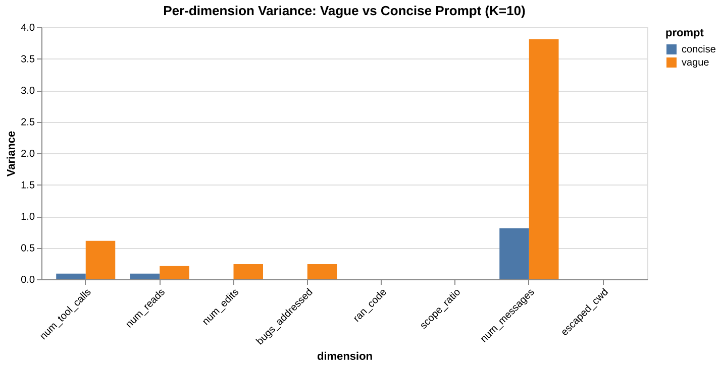
The chart shows most of the vague prompt’s width comes from num_messages (3.81 vs 0.81). The concise prompt squashes it by nearly 5x. Both prompts have zero variance on ran_code, scope_ratio, and escaped_cwd. The task structure determines those dimensions, not the prompt. The variation concentrates in effort: how many messages and tool calls it takes.
If we wanted to keep the prompt flexible but reduce width, the data points at message count as the dimension to constrain. Perhaps a tighter stopping criterion rather than a different prompt entirely.
Convergence — are outcomes stable?
Width told us there is behavioral variation. But variation is only a problem if it affects outcomes: a wide Field where every run succeeds is fine; a narrow Field with random outcomes might not be.
Convergence separates these cases. It measures the signal-to-noise ratio of outcomes, mean divided by standard deviation.
m.convergence() # 1.22
High convergence: outcomes are consistent within the behavioral space we defined. Low convergence: outcomes are unstable. The mean might look decent, but any individual run is a coin flip.
Convergence is scoped to the Field we built. If our $\varphi$ misses a critical behavioral axis, convergence could be high and the agent could still be failing in ways the Field cannot see.
If convergence is high, we may be done. There is variation (width told us that), but it does not affect outcomes. If convergence is low, something in the behavioral space we are measuring is unstable, and we need to find what. That is the next question.
Pass rate vs convergence
From the prompt ablation experiment above:
vague_field.metrics().convergence()    # 1.22  (6/10 pass)
concise_field.metrics().convergence()  # inf   (10/10 pass)
The jump from 1.22 to $\infty$ is invisible in pass rate (0.6 to 1.0). But the operational difference is significant. The vague Field has high outcome variance within the measured behavioral space: 6 out of 10 pass, but which 6 is not predictable from the prompt alone. The concise Field has zero outcome variance. Whether that translates to production reliability depends on whether the $\varphi$ captured the right dimensions, but the signal within the Field is unambiguous.
Convergence is the first thing to check when comparing configurations. If we change the prompt and convergence goes up, outcomes have become more consistent along the dimensions we chose to measure. If it goes down, we have introduced instability in the dimensions the Field is constructed with.
Separation — what distinguishes success from failure?
Convergence told us outcomes are unstable. Now we need to know which dimensions separate the successes from the failures. Not all dimensions will matter. Some will be identical across both groups. The ones that differ are where the problem lives.
The vector between the centroid of successful trajectories and the centroid of failures:
m.separation()
# array([-1.33, -0.33, -1.0, -1.0, 0.0, 0.0, -3.0, 0.0])
#        ↑ tool_calls    ↑ edits          ↑ num_messages
#        successes        successes        successes used
#        used fewer       made fewer       far fewer messages
Each component says how much the two groups differ on one dimension. Large positive means successes scored higher. Large negative means successes scored lower. Near zero means that dimension does not distinguish the groups.
Separation points at the problem. num_messages (-3.0) is the loudest signal: successes averaged 16 messages, failures averaged 19. num_edits (-1.0) is sharp: every success made exactly 3 edits, every failure made 4. Three dimensions (ran_tests, scope_ratio, escaped_cwd) show zero separation. Both groups did the same thing on those axes. They are not where the problem lives.
But separation only tells us that dimensions differ. It does not tell us what to do about it. If num_messages separates the groups, should we give fewer messages (constrain the search) or more (expand the budget)? We need to know the direction.
Reading a separation chart
from agent_fields.visualisations import separation_bar
chart = separation_bar(m)
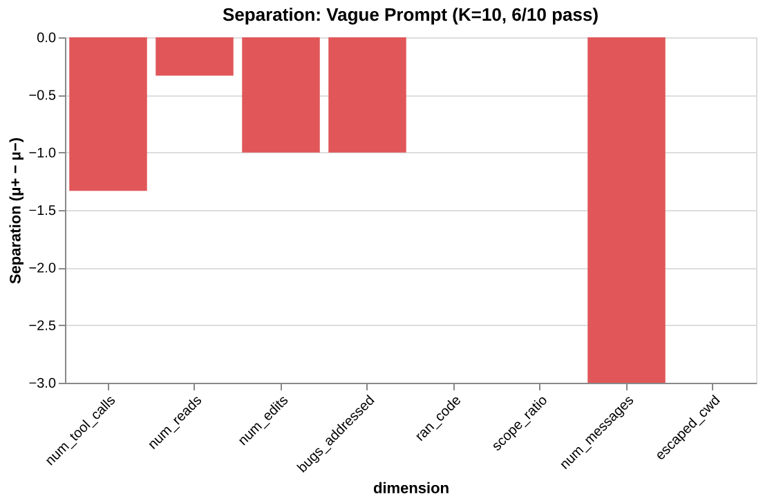
The separation chart paints each dimension green (successes higher) or red (successes lower). From the vague-prompt Field (K=10, 6/10 pass):
| Dimension | Separation | Reading |
|---|---|---|
num_tool_calls |
-1.33 | Successes used fewer calls |
num_reads |
-0.33 | Slight difference. Not diagnostic |
num_edits |
-1.00 | Successes made exactly 3 edits. Failures made 4. |
bugs_addressed |
-1.00 | Failures touched more bug-related code |
ran_tests |
0.00 | Both groups ran tests |
scope_ratio |
0.00 | Both groups stayed on target |
num_messages |
-3.00 | Successes used far fewer messages |
escaped_cwd |
0.00 | No difference |
The story the separation vector tells: failing trajectories did more work, not less. They made more edits, used more tool calls, spent more messages. They were not under-resourced. They over-worked the problem, making a 4th edit where 3 sufficed, using extra messages to revise and retry. The signal suggests the intervention is not “give more turns” but “make the prompt more specific so the search converges in fewer steps.”
Pass rate says “4 out of 10 failed.” Separation tells us what the failures did differently, across every dimension, in one vector.
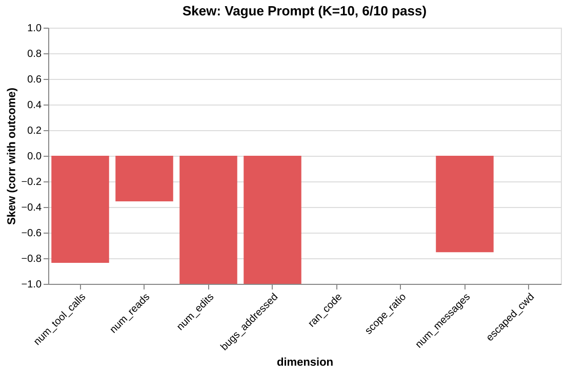
Skew — on the flagged dimensions, does more help or hurt?
Separation flagged the dimensions. Skew tells us the direction on each one. It is the correlation between outcome and one behavioral dimension:
m.skew("num_edits")       # -1.0 — more edits correlates with failure
m.skew("num_tool_calls")  # -0.84 — more tool calls correlates with failure
m.skew("num_reads")       # -0.36 — weak signal
A number between -1 and +1. Negative: doing more on this dimension correlates with failure. Positive: doing more correlates with success. Near zero: no relationship.
This is where the diagnostic becomes an intervention. Negative skew on num_edits (-1.0) means the failing trajectories over-edited. The fix is not “allow more edits.” It is to help the search converge on the right edit the first time. Positive skew on num_edits would mean the opposite: the agent needs more room to edit, give it budget.
Here, every skew signal is negative. The failures are not struggling from lack of resources. They are doing too much. The intervention is to constrain, not expand.
Reading skew on each flagged dimension
Negative skew on num_edits (-1.0): Every trajectory that made 3 edits succeeded. Every trajectory that made 4 edits failed. Perfect negative correlation. The failing trajectories made an extra edit, likely revising their first fix or introducing a regression they then attempted to repair.
Negative skew on num_tool_calls (-0.84): Trajectories that made fewer tool calls tended to succeed. Consistent with the num_edits story: the failing trajectories used more tools without making better progress. They were not under-resourced. They were thrashing.
Weak skew on num_reads (-0.36): Reading more files has a slight negative correlation with success. Not the bottleneck. Do not optimize it.
Visualizing skew
from agent_fields.visualisations import skew_bar
chart = skew_bar(m)
The chain
Width → convergence → separation → skew. Each step narrows the question. Width asks “is there variation?” Convergence asks “does the variation matter?” Separation asks “where does it matter?” Skew asks “what do I do about it?”
The workflow: check convergence (is there a problem?), read separation (where?), check skew on the flagged dimensions (constrain or expand?), intervene, then build the new Field and compare.
The Field is not static
Everything above operates on the point cloud of completed trajectories. K trajectories, measured at completion. The metrics tell us what the trajectories did and how well they did it. But they do not tell us when things went right or wrong.
The previous essay described the Field shifting with every token as context accumulates. “Long-task failure is drift, not confusion.” The agent does not suddenly fail at step 40. It accumulates noise through the context window, and the Field warps gradually until the search lands in the wrong place.
This is a temporal claim. The point cloud — one point per completed trajectory — cannot answer it. A completed trajectory has been projected to a single point; the progression that produced it is gone.
We need a second lens. Not a replacement for $\varphi$, but a complement. Where $\varphi$ asks what did the agent do?, this new lens asks where in the task is the agent?
The state function
We call this $\psi$ (psi). It takes a trajectory and a position in that trajectory, and returns a discrete label representing semantic progress.
The true state at any moment is the full context window: every observation, every action, every token accumulated so far. That is intractable. $\psi$ compresses it into a human-legible label: “start”, “diagnosed”, “editing”, “complete_fix”, “tested.” The compression is lossy by design. We choose what aspects of progress matter and discard the rest.
The progression is linear. The task has a logical ordering: diagnose before fixing, fix before verifying. Different trajectories traverse this at different speeds, with different behaviors at each state, but the progression itself is a line. States are monotonic.
In the same Field subclass, $\psi$ is the
class CodeFixField(Field):

    def dimensions(self): ...   # phi — what did the agent do?
    def measure(self, trajectory): ...

    def trajectory_length(self, trajectory):
        return len(trajectory["messages"])

    def state(self, trajectory, t):
        """psi — where in the task at step t?"""
        messages = trajectory["messages"][:t + 1]
        tool_calls = extract_tool_calls(messages)

        has_read_buggy = any(
            tc["name"] == "Read" and "buggy" in str(tc.get("input", {}).get("file_path", ""))
            for tc in tool_calls
        )
        has_edited = any(tc["name"] == "Edit" for tc in tool_calls)
        bugs_fixed = count_bugs_addressed(tool_calls)  # checks edit content
        has_tested = any(
            tc["name"] == "Bash" and "python" in str(tc.get("input", {}).get("command", ""))
            for tc in tool_calls
        )

        if not has_read_buggy:       return "start"
        if not has_edited:           return "diagnosed"
        if bugs_fixed < 3:           return "editing"
        if not has_tested:           return "complete_fix"
        return "tested"
state() takes the trajectory and a step index t. It looks at everything up to step t, checks which milestones have been reached, returns the most advanced one. Five states: start → diagnosed → editing → complete_fix → tested. The gates are sequential: each requires the previous.
tells the framework how many steps to evaluate. At ingestion time, the Field calls state(trajectory, t) for every t, recording the full state sequence. This happens once per trajectory at
The critical design choice in state() is what counts as progress. A naive version might check “has any Edit been made.” The version above checks what the edit actually did: count_bugs_addressed inspects whether the edit content modifies the buggy function definitions, not just whether an edit occurred. A trajectory that edits test inputs instead of function bodies stays at "editing", not "complete_fix". This distinction is what produces horizon variation: in the Haiku experiment, 5 out of 19 trajectories that made edits never addressed the actual bugs.
$\psi$ and $\varphi$ are orthogonal. They sit on the same trajectory but answer different questions:
state() — $\psi$ |
measure() — $\varphi$ |
|
|---|---|---|
| Asks | Where in the task? | What is the behavior? |
| Returns | Discrete label | Vector in $\mathbb{R}^d$ |
| Captures | Semantic progress | Strategy, cost, variation |
| Example | "editing" |
[calls=7, reads=3, edits=1, bugs=0] |
The state says “the trajectory is editing but has not fixed the bugs.” The measurement says “it made 7 tool calls, read 3 files, produced 1 edit, addressed 0 bugs.” Together: where and how.
Behavioral variation within a state (“during editing, did the trajectory fix the function or the test inputs?”) is captured by measure(), not by subdividing state(). State stays coarse and linear. Measurement stays high-dimensional and detailed.
How state() labels a trajectory at each step
A single trajectory, 12 steps. The Field calls state(trajectory, t) for t in range(12):
| Step | Action | state(trajectory, t) |
|---|---|---|
| 0 | Read task description | "start" |
| 1 | List files in directory | "start" |
| 2 | Read buggy.py |
"diagnosed" |
| 3 | Read test_buggy.py |
"diagnosed" |
| 4 | Analyze the divide-by-zero bug | "diagnosed" |
| 5 | Edit buggy.py: fix divide() |
"editing" |
| 6 | Edit buggy.py: fix average() |
"editing" |
| 7 | Edit buggy.py: fix first_element() |
"complete_fix" |
| 8 | Run python buggy.py |
"tested" |
| 9 | Tests pass | "tested" |
| 10 | Read output | "tested" |
| 11 | Report completion | "tested" |
Stored sequence: ["start", "start", "diagnosed", "diagnosed", "diagnosed", "editing", "editing", "complete_fix", "tested", "tested", "tested", "tested"].
A different trajectory might fix all three bugs in a single edit, jumping from "diagnosed" to "complete_fix" in one step. Another might make edits that never address the real bugs, staying at "editing" until it runs out of turns. Different state sequences, but all are comparable through horizons: among all trajectories that reached "complete_fix", what does the point cloud of their behavioral measurements look like?
state() is also a hypothesis
Just as measure() is our hypothesis about which behavioral properties matter, state() is our hypothesis about which states matter.
For code-fixing: start → diagnosed → editing → complete_fix → tested. This says the critical transitions are finding the target file, beginning to edit, fixing all the bugs, and running tests.
Someone else studying the same trajectories might define: start → exploring → committed → done. Different compression, different horizons, different insights.
A third person might care about one transition:
class MinimalField(Field):
    def state(self, trajectory, t):
        has_tested = any_test_calls_up_to(trajectory, t)
        return "after_tests" if has_tested else "before_tests"
Two states. One question: does running tests change the Field?
There is no correct state(). There is the one that answers our question. Like measure(), work backwards from the decision.
Horizons
state() labels each step of a trajectory. A Field to only trajectories that passed through a given state. It is itself a Field, with the same dimensions, outcome labels, and full metrics, but scoped to trajectories that reached a particular state.
h = field.horizon("diagnosed")

h.K                       # 18 — trajectories that reached diagnosis
h.metrics().width()       # 5.3 — behavioral spread among those 18
h.metrics().convergence() # 1.8 — outcome consistency for that group
h.metrics().separation()  # separation within this group
horizon("editing") does not measure what the agent was doing during editing. It is the point cloud of behavioral measurements — the full measure() output — filtered to trajectories that passed through "editing" at some point. Same points, smaller set.
But this is not a limitation. The full Field is already an approximation: K samples from the true distribution over behaviors. Each horizon is the same kind of approximation, conditioned on a state. The full Field approximates “what does the agent do from the start?” The horizon approximates “what does the agent do, given it reached this state?” Filtering trajectories by state and measuring the resulting cloud is the same sampling logic, just conditional.
And because states are monotonic, conditioning on “editing” implies that everything before it was covered: the agent read the target file (diagnosed), it began making edits. The pre-editing history is baked into the gate. What varies among trajectories in this horizon is what happened from that state onward. The shared prefix is guaranteed by the state progression; the divergence is downstream.
Every metric works on it. We can compute separation within a horizon: among trajectories that reached editing, what distinguishes the ones that ultimately succeeded?
Because states are monotonic, horizons nest:
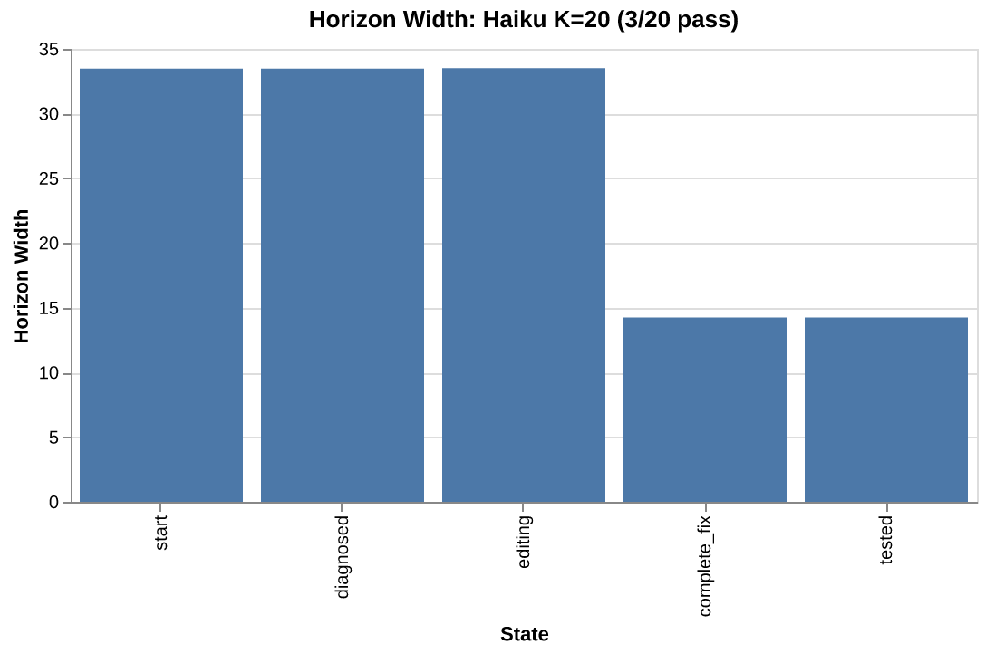
The horizon at “start” is the full Field. Walking the chain, computing metrics at each state, shows how the point cloud of behavioral measurements changes as we condition on progressively deeper progress:
for s in field.states:
    h = field.horizon(s)
    hm = h.metrics()
    print(f"{s:>12}: K={h.K:>2}  width={hm.width():.1f}  conv={hm.convergence():.2f}")
This data comes from running the
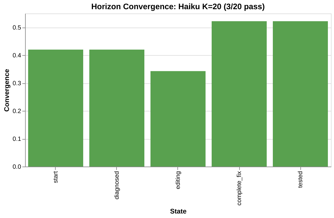
       start: K=20  width=33.5  conv=0.42
   diagnosed: K=20  width=33.5  conv=0.42
     editing: K=19  width=33.5  conv=0.34
complete_fix: K=14  width=14.2  conv=0.52
      tested: K=14  width=14.2  conv=0.52
Read it as progressive filtering: all 20 trajectories passed through start. All 20 also reached diagnosed: every one read the buggy file. 19 reached editing (all but one made at least one edit). But only 14 reached complete_fix: only 14 produced edits that addressed all three bugs. The other 5 made edits that touched call sites or test inputs instead of the actual function definitions.
The biggest drop, editing to complete_fix, is the critical gate. Width drops from 33.5 to 14.2. The 5 trajectories that never produced correct edits are excluded, and the remaining cloud is dramatically tighter.
Notice that start and diagnosed are identical (K=20 both). Every trajectory reads the target file. Conditioning on diagnosis does not change the cloud at all. The variation lives downstream, in what the agent does after reading.
But the horizon chain shows narrowing. It does not distinguish whether that narrowing is healthy (good trajectories converging on a strategy) or problematic (failures diverging from successes). Both look like width dropping and K shrinking. To separate these two stories, we need one more tool.
Horizons are composable with the diagnostic chain
Every horizon is a Field. The diagnostic chain works inside it:
diag = field.horizon("diagnosed")
dm = diag.metrics()

dm.convergence()          # 0.42 — low, same as the full `Field` here
dm.separation()           # which dimensions separate success/failure among diagnosed trajectories?
dm.skew("bugs_addressed") # among these trajectories, does coverage correlate with outcome?
This is the same chain (convergence, separation, skew) applied to a subset. The question changes from “what distinguishes success from failure across all runs?” to “among trajectories that reached diagnosis, what distinguishes the ones that ultimately succeed?”
Different horizons reveal different stories. Separation at "editing" flags bugs_addressed (+1.06): successes addressed more bugs. Separation at "complete_fix" flags num_messages (-3.0) and num_edits (-1.85) instead: among trajectories that fixed all bugs, failures used more messages and more edits. The failure mode shifts depending on which gate we condition on.
Grouping fine-grained states at query time
When state() returns fine-grained labels, group them at query time:
# Multiple state labels treated as one
h = field.horizon(["debugging:core_files", "debugging:tests", "debugging:logs"])
state() stays unchanged. Define at full resolution, select at analysis time. This keeps the state function simple and lets us slice differently for different questions.
Visualizing horizons
from agent_fields.visualisations import horizon_width, horizon_convergence

horizon_width(field)
horizon_convergence(field)
Drift
Horizons show the Field narrowing as trajectories progress through states. But narrowing is ambiguous. Width drops from 33.5 at start to 14.2 at complete_fix. Is that because successes are clustering tightly (good) or because failures are scattering away from the success corridor (bad)?
Drift separates these two stories. At each state, compare the width of all trajectories in that horizon to the width of only the successful ones:
If successes are tight and the full horizon is wide, the difference is the extra spread that failures contribute. That difference is drift.
for s in field.states:
    h = field.horizon(s)
    W_all = h.metrics().width()
    sr = h.success_region()
    W_success = sr.metrics().width() if sr.K >= 2 else W_all
    print(f"{s:>12}: drift={W_all - W_success:.2f}")
From the Haiku K=20 experiment:
       start: drift=17.69   (K+=3)
   diagnosed: drift=17.69   (K+=3)
     editing: drift=33.01   (K+=2)
complete_fix: drift=-1.53   (K+=3)
      tested: drift=-1.53   (K+=3)
Look at the K+ column. Drift at editing is 33.01, but it is computed from 2 successful trajectories. That is not a success corridor. That is two points. The number comes out of the formula, but it carries no statistical weight. The same problem exists at every horizon: K+=3 is barely better. With so few successes, the within-model drift calculation is unreliable.
This is a common situation. Weak models on hard tasks produce few successes. The very runs where drift analysis would be most useful are the ones where the
Using a baseline Field as a ruler
A Field can be used as a ruler. Build a reference corridor from a capable model’s success region (or from curated golden runs, or human-operated traces), and measure any other model’s trajectories against it. The reference corridor does not have to come from the same model, or even the same kind of source. It only needs enough successful trajectories to define a stable region in the behavioral space the Field prescribes.
This solves the drift problem from above. Within-model drift requires enough successes to define a stable success corridor, and weak models on hard tasks produce few successes. A cross-model baseline sidesteps this entirely: use a strong model’s success corridor as the ruler, and measure the weak model’s trajectories against it at every horizon.
Example: Sonnet success corridor as a ruler for Haiku
We ran the same bug-fixing task with both Sonnet (K=20, 13/20 pass) and Haiku (K=20, 3/20 pass), using the same Field.
sonnet = build_field(sonnet_run)
haiku = build_field(haiku_run)

# Sonnet success corridor — the ruler
baseline = sonnet.success_region()
baseline.K              # 13
baseline.metrics().width()  # 2.60 — stable across all horizons
Compare Haiku’s trajectories at each horizon against this baseline:
for s in haiku.states:
    h = haiku.horizon(s)
    W_haiku = h.metrics().width()
    W_baseline = baseline.metrics().width()
    print(f"{s:>12}: W_haiku={W_haiku:.1f}  W_baseline={W_baseline:.1f}  gap={W_haiku - W_baseline:.1f}")
       start: W_haiku=33.5  W_baseline=2.6  gap=30.9
   diagnosed: W_haiku=33.5  W_baseline=2.6  gap=30.9
     editing: W_haiku=33.5  W_baseline=2.6  gap=30.9
complete_fix: W_haiku=14.2  W_baseline=2.6  gap=11.6
      tested: W_haiku=14.2  W_baseline=2.6  gap=11.6
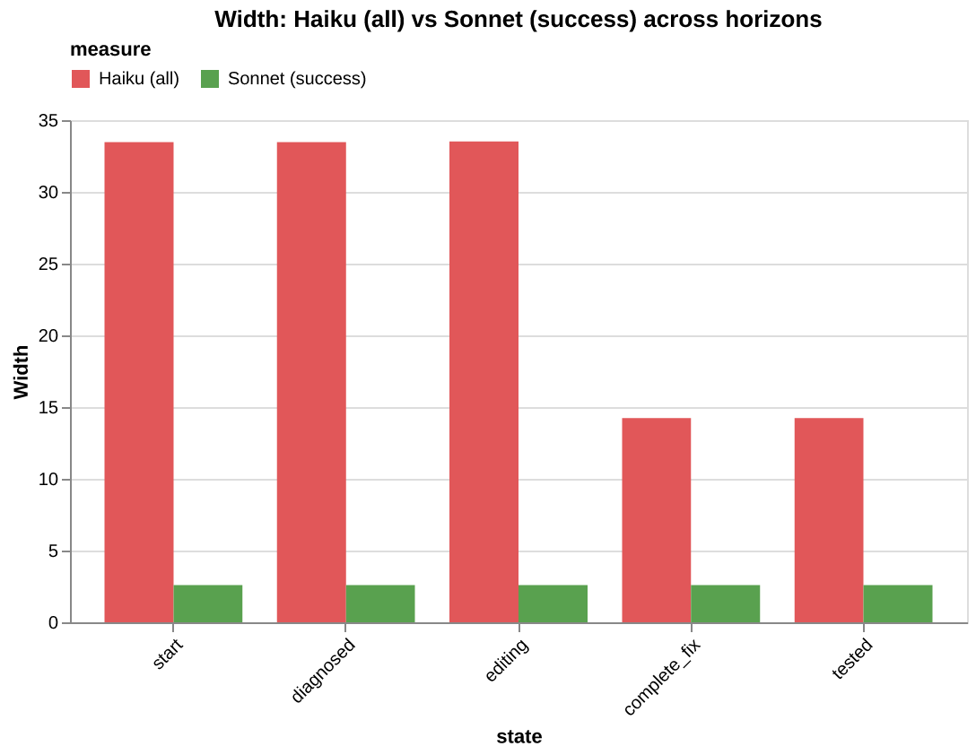
Haiku is 10-13x wider than the success corridor at every state. The gap drops at complete_fix (30.9 → 11.6) when the 5 trajectories that edited the wrong things are filtered out. But even the 14 that addressed all bugs are still far outside the corridor.
The centroid gap reveals where in behavioral space Haiku lands relative to the corridor:
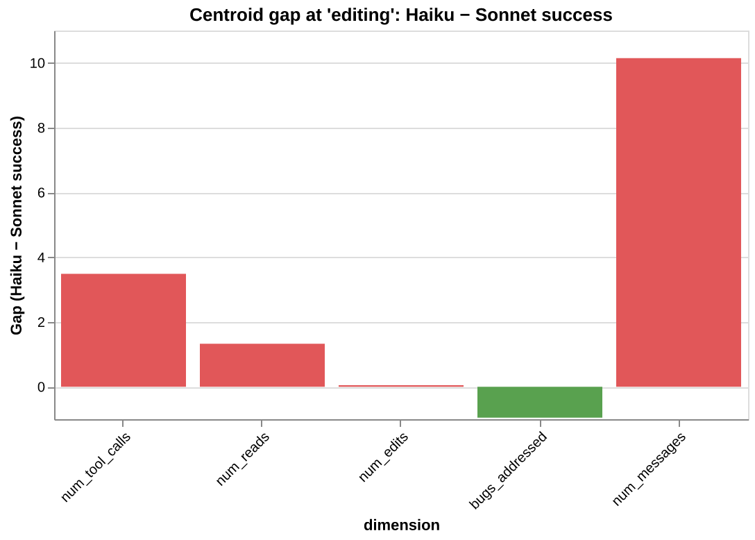
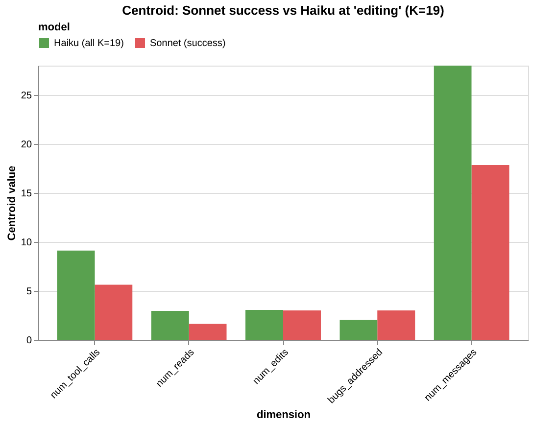
At editing (K=19): Haiku does more work on every dimension — 55% more messages, 60% more tool calls — but addresses fewer bugs. The diagnosis: Haiku’s problem is not resource starvation. The trajectories are editing the wrong things.
At complete_fix (K=14), the gap changes character. The bugs_addressed gap disappears (by definition, all 14 addressed all 3 bugs). But the num_messages gap grows to +12.5, and num_edits appears at +0.79. Even the Haiku trajectories that produced correct fixes needed an extra edit and 12 more messages to get there.
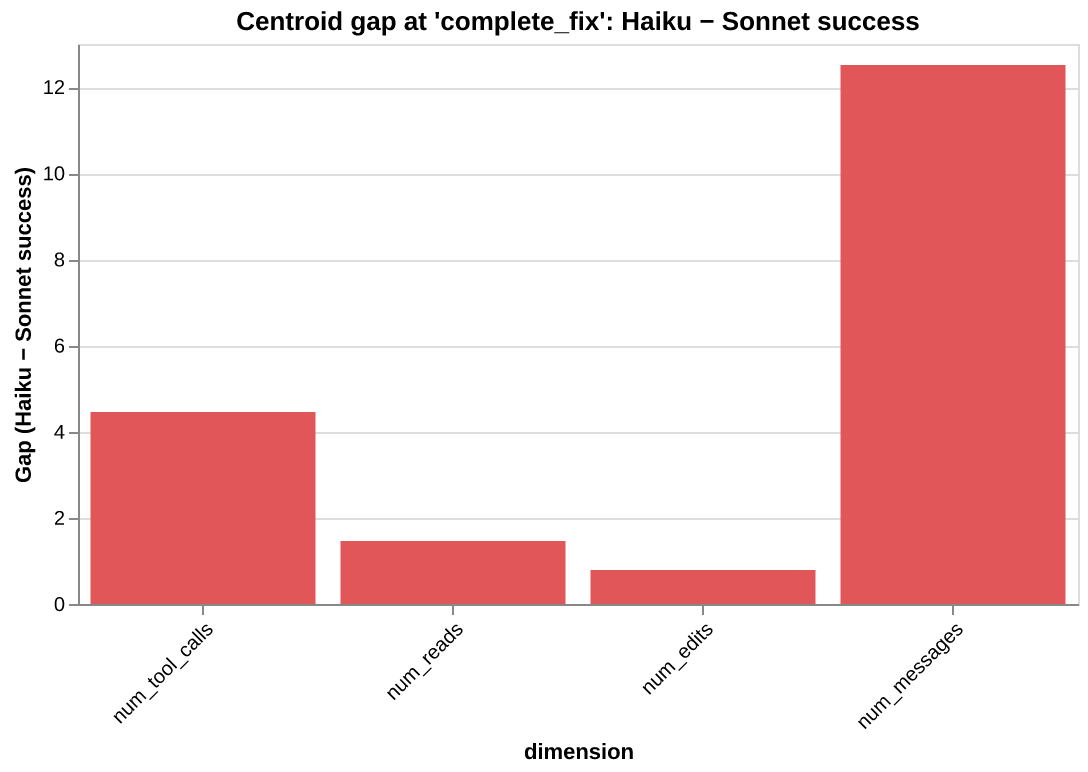
The failure mode shifts depending on which state we condition on. At editing, it is about targeting (wrong bugs). At complete_fix, it is about efficiency (right bugs, more effort). Horizons reveal this shift; the baseline corridor gives stable ground to measure it from.
Intent: what was the policy doing?
The ruler showed Haiku is far from the success corridor. Drift showed where. But neither answers the question that actually matters for engineering: what was the policy doing differently?
Two trajectories can land at the same state with similar $\varphi$ measurements (same number of tool calls, same scope ratio) but one is confidently executing while the other is recovering from a failed attempt. $\varphi$ can’t see this because it erases temporal order. $\psi$ can’t see this because both are at the same task state. The policy’s operational character, the thing that determines what happens next, is invisible to both lenses.
We need a third lens. One that reads not the task’s signal in the trajectory (that’s $\psi$), but the policy’s signal.
The intent function
Intent ($\rho_\pi$) is a user-defined function that labels each trajectory step with a discrete marker:
where $\mathcal{I}$ is a finite alphabet of intent labels. Unlike $\psi$, intent is non-monotonic. The policy can move between labels in any order, revisiting earlier operational modes.
| $\psi$ (state) | $\rho_\pi$ (intent) | |
|---|---|---|
| Serves | the trajectory | the policy |
| Monotonic | yes, progress only moves forward | no, the policy can revisit modes |
| Reads | task milestones | operational character |
| Question | where did the task get to? | how was the policy operating? |
For the bug-fixing task, we use the simplest meaningful decomposition: binary intent.
- acting: the model makes tool calls (Read, Edit, Bash, Glob, …)
- introspecting: the model produces reasoning tokens with no tool calls
This is a coarse lens. Richer labels (orienting, executing, recovering, …) are possible and would enable more fine-grained analysis. But binary is enough to reveal structural differences across models.
class IntentFluctuationField(aft.Field[dict]):
    """Field with three lenses: measure (φ), state (ψ), intent (ρ_π)."""

    def intent(self, trajectory: dict, t: int) -> str:
        msg = trajectory["messages"][t]
        if is_assistant(msg):
            if has_tool_calls(msg):
                return "acting"
            if has_text(msg):
                return "introspecting"
        # non-assistant messages inherit from the nearest assistant
        ...
The full implementation is in
Semantic chains
With intent defined, we can look at the semantic sequence of each trajectory: the full action trace interleaving tool names with model_introspection labels showing where the model reasoned between actions.
We ran K=20 trajectories for each of three models: Haiku, Sonnet, and Opus. The
OPUS   (20/20 pass)
   Glob → Read → MI → Edit×3 → MI → Read → Bash → MI

SONNET (13/20 pass)
   MI → Read → MI → Edit×3 → MI → Bash → MI → Read → MI     ← passes
   MI → Read → MI → Edit×4 → MI → Bash → MI → Read → MI     ← fails

HAIKU  (3/20 pass)
   MI → Read → MI → Bash → MI → Read → MI → Edit×4 → MI → Read → MI → Bash → MI
   MI → Read → MI → Bash → MI → Read → MI → Bash → MI → Edit → MI → Read → MI → Edit×4 → ...
Three observations:
- Opus starts by acting (
Glob → Read, no leading MI). Sonnet and Haiku start by introspecting (MI → Read). - Sonnet has two modes.
Edit×3runs pass;Edit×4runs fail. The fourth edit is the signal: the model misidentified a bug. - Haiku’s chains vary significantly across runs. More back-and-forth between acting and reasoning. It interleaves Bash and Read throughout, using test feedback to guide its next action rather than working from a diagnosis.
Program strings and program families
Run-length encoding the intent sequence produces a program string, the compressed behavioral fingerprint of the trajectory. Each trajectory maps to a sequence of alternating acting/introspecting runs.
The Field’s program_family() groups trajectories that share the same program string. This partitions the field by structural similarity: trajectories in the same family followed the same act/think pattern regardless of what specific tools they called or what files they targeted.
for prog in field.programs:
    fam = field.program_family(prog)
    fm = fam.metrics()
    short = " → ".join(p[0].upper() for p in prog)   # A/I
    print(f"  {fam.K:>2}× (pass={wins}/{fam.K}, width={fm.width():.2f})  {short}")
Here is what fell out of the data:
| Model | Distinct programs | Act/think cycles | Pass rate | Field width |
|---|---|---|---|---|
| Opus | 1 | 3 | 20/20 | 3.94 |
| Sonnet | 2 | 4–5 | 13/20 | 1.06 |
| Haiku | 5 | 6–10 | 3/20 | 8.69 |
Program count increases as capability decreases. Opus produces one program across all 20 runs. Sonnet splits into two. Haiku fragments into five. Cycle count follows the same pattern: Opus alternates 3 times, Haiku up to 10.
Within-family width reveals a second dimension of variation. Opus has one program but width=3.94: same alternation pattern, different tool arguments across runs. Sonnet’s dominant family has width=0.66, its passing trajectories tightly clustered in behavioral space. Haiku’s largest family has width=6.98. Even runs that share a program diverge in their behavioral vectors.
The
Conclusion
summary of everything until now
The construction rests on three lenses over the same trajectory. measure() projects what the agent did into a point cloud, the empirical Field. state() labels where in the task each step falls, slicing that cloud into horizons. intent() labels how the policy was operating at each step, compressing the trajectory into a program string. Every metric (width, convergence, separation, skew) works on all three.
| Object | Python | What it gives us |
|---|---|---|
| $\varphi$ | field.measure(trajectory) |
K points in d-dimensional space |
| $\psi$ | field.state(trajectory, t) |
State labels along each trajectory |
| $\rho_\pi$ | field.intent(trajectory, t) |
Intent labels along each trajectory |
Field |
field.points, field.outcomes |
The empirical search space |
| Metrics | field.metrics() |
Width, convergence, separation, skew |
| Horizons | field.horizon("editing") |
Metrics scoped to a state |
| Drift | $W_{\mathcal{H}(s)} - W_{\mathcal{H}^+(s)}$ | Where failures depart from the success corridor |
| Regions | field.success_region() |
The cloud partitioned by outcome |
| Programs | field.programs |
Distinct behavioral programs across trajectories |
| Program Families | field.program_family(prog) |
Sub-field scoped to trajectories sharing a program |
The metrics:
- Width — is the measured behavior constrained or scattered across the dimensions you defined?
- Convergence — are outcomes consistent within the behavioral space you chose to measure?
- Separation — along which measured dimensions do successful and failing trajectories differ?
- Skew — on a given dimension, does doing more correlate with success or failure?
- Horizons — at which state does the measured behavioral variation change?
- Drift — at which state do failing trajectories diverge from the success corridor within your
Field?
The previous essay told us the Field exists. That the prompt narrows it, the environment bounds it, feedback steers it, noise warps it. Now each claim has a measurement:
| Claim from the previous essay | Measurement |
|---|---|
“The prompt narrows the Field” |
Compare widths across prompts |
| “Feedback steers the search” | Compare convergence with and without test suites |
| “Long-task failure is drift” | Walk the horizon chain. Find where drift spikes |
| “The environment bounds the search” | Change the environment. Compare both fields |
| “Two identical clouds can hide different strategies” | Compare program distributions across models |
What this enables
Three lenses, one trajectory:
- $\varphi$ sees what happened: the behavioral vector
- $\psi$ sees where the task got to: progress through states
- $\rho_\pi$ sees how the policy operated: the program it executed
The Field subclass is a behavioral prescription anchored to the task, not the model. It defines which dimensions matter and which states define progress. That prescription is model-independent. Any model that runs the same task through the same Field produces points in the same behavioral space. This makes the Field a ruler: build a reference corridor from a capable model’s success region, and measure any other model against it.
The vocabulary and its objects are not confined to one tool or one library. The objects ($\varphi$, $\psi$, $\rho_\pi$, the cloud, the metrics) are abstractions that can be implemented in any stack, applied to any agent, measured on any task. The Python library is one form of expression. The school of thought is what matters: treat agent behavior as a distribution. Measure the distribution’s shape. Use the shape to make engineering decisions.
The tutorials that accompany this essay put the vocabulary and objects to work on simulated scenarios.
This framework does not predict what an agent will do. As stated throughout the essay, the
Fieldis an empirical instrument, not a generative theory. We cannot derive the true distribution over trajectories from first principles. What we can do is define a proxy: a set of dimensions and states that capture the behaviors we care about, and then measure whether the agent lives within them.
That proxy is subjective by design. The Field does not describe the full space of reachable behaviors. It describes the space we chose to look at. measure() is our hypothesis about what matters. state() is our hypothesis about what progress looks like. The framework tests those hypotheses. We change a prompt, swap a model, modify the environment, and the Field tells us whether the behavioral distribution shifted in the directions our dimensions can see. Everything works backwards: start from the behaviors we expect, define the dimensions that would reveal them, then run the experiment.
This implies something deeper than just “test the agent.” It means thinking not only about what the agent should achieve, but about the space of programs it might construct along the way. This is the fundamental difference between LLM software and traditional software. Traditional software is statically baked. Line 5 of a program executes whatever instruction was written on line 5. No matter how dynamic the runtime graph, no instruction is synthesized out of thin air. LLM-based software breaks this invariant. The agent’s next action is sampled from a distribution. Line 5 could be a completely different program on every run. The code is not written; it is searched for, live, conditioned on everything that came before.
Given the entropy in those unrolled trajectories, reasoning about agent behavior without measurement is guesswork. The framework makes it empirical. And because the Field is defined by us, not by the model provider, it enables something practical: behavioral alignment metrics. We define the behavioral prescription, the dimensions and states that describe how the agent should behave, and then measure how consistently any model adheres to it. The focus shifts from refining what the prompt says to prescribing what the behavior should look like, and then holding the system accountable to that prescription across models, prompts, and environments.
Where can you use this
This framework applies broadly across the ML/AI domain because all it does is map trajectory space to a behavioral space. That transformation buys us a language for measuring abstract behaviors, and that language opens several doors:
- Model alignment studies
- Long-horizon task analysis
- Using the
Fieldas a reward function (optimization target) - Using the
Fieldas an empirical foundation for prompt ablation studies